OBIEE - Formatting Calculated Items in a Pivot Table

I have been spending a lot of time with OBIEE and Essbase lately (quite often much more time than should have been necessary!) and so my first blog in much too long is about my latest hurdle. It seems that OBIEE is full of hurdles and sneaky workarounds (and also some amazing customisation/extension opportunities using third party visualisations). Using Essbase and OBIEE together probably exponentially increases the amount of hurdles but I am still enjoying the product.

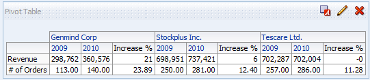
I recently wanted to create a table with measures in the rows and years and organisations in the columns. I also wanted to have a increase % column added.

e.g.

	Genmind Corp			Stockplus Inc.			Tescare Ltd.
	FY13	FY14	Increase %	FY13	FY14	Increase %	FY13	FY14	Increase %
Revenue	298,762	360,576	21%	698,951	737,421	6%	702,287	702,004	0%
# of Orders	113	140	24%	250	281	12%	257	286	11%

This seemed easy enough to do using a calculated item on the Fiscal Year column in the table.

It quickly became apparent however that the formatting options are very limited for this new column. Basically you only get style formatting and cannot change the number format and therefore you cannot choose to display the output as a percentage.

A quick thinker might instantly just try to concatenate a percentage sign onto the end of the number but would be even more quickly disappointed when the editor only allows numerical calculations/output.

The solution is not particularly convoluted thankfully. All you need to do is add a conditional format onto each of your measure fields with the condition that when the column ('Per Name Year') is null, then apply the percentage data format. So the steps are:

1. Go back to the criteria tab
2. Edit the column properties for the 'Revenue' column and click on the Conditional Formatting tab.
3. Click Add Condition and select 'Per Name Year'
4. Select Operator "is null' and press OK
   
5. Select your formatting options. I have selected the 'Data Format' tab and selected Override, Percentage, Parantheses (red).
   
6. Select OK and you should see something like the following screenshot.
   
7. Navigate to the Results tab and you will see the result.
   

Notice that the second measure is still not formatted (# of Orders). You will need to repeat the conditional formatting on every measure.

The final result will be:

It should be noted that this would only work if you only had a single calculated column or you wanted all your calculated columns to have a single format.

There you have it. Hopefully that gets someone out of a bind. I would be keen to hear any other options people use, especially if they are better! I'm sure another option would be to modify the XML which would work for different formatting on multiple calculated columns.